Scaling to 2 Trillion Tokens a Day

One customer asked us if we could serve them 2 trillion tokens a day of MiniMax M3.1 Flash. We said yes, and made it a reality. In this post, we’ll walk through the system design decisions, the inference optimizations, and how we stress-tested a workload this size.

To put 2 trillion tokens a day at scale, if this was an individual model on OpenRouter, it would be the fourth-largest model on the platform, with nearly twice the traffic of Claude Opus 5.5. That’s the entire text of English Wikipedia, about 5 billion words, roughly 300 times over, every day.

At peak, that means:

• 550 requests per second
• 5,000 requests in flight at once
• 756 AMD MI325X GPUs serving it

OpenRouter rankings, data through Oct 29, 2026.

At Featherless, we support over 40,000 open-source models, all usable from one API key. Most of that traffic is spread over thousands of models. This customer gave us a different challenge: scaling an enormous amount of traffic across just one model.

Very few teams serve an open model at this scale, and even fewer do it on AMD hardware.

Understand your data

The customer told us that the majority of the traffic would be agentic coding. These details are very important. The way you optimize your inference stack depends heavily on the shape of the data being sent. Compare a customer-support chatbot on a small business website to an autonomous coding agent: they have completely different needs.

The data structure behind agentic coding is a conversation tree, where each node can be a bash command, a tool call, a text response, and so on. Every turn sends the conversation so far, plus whatever is new. That’s very well suited to caching, so we spent a lot of time designing an inference stack that takes advantage of it.

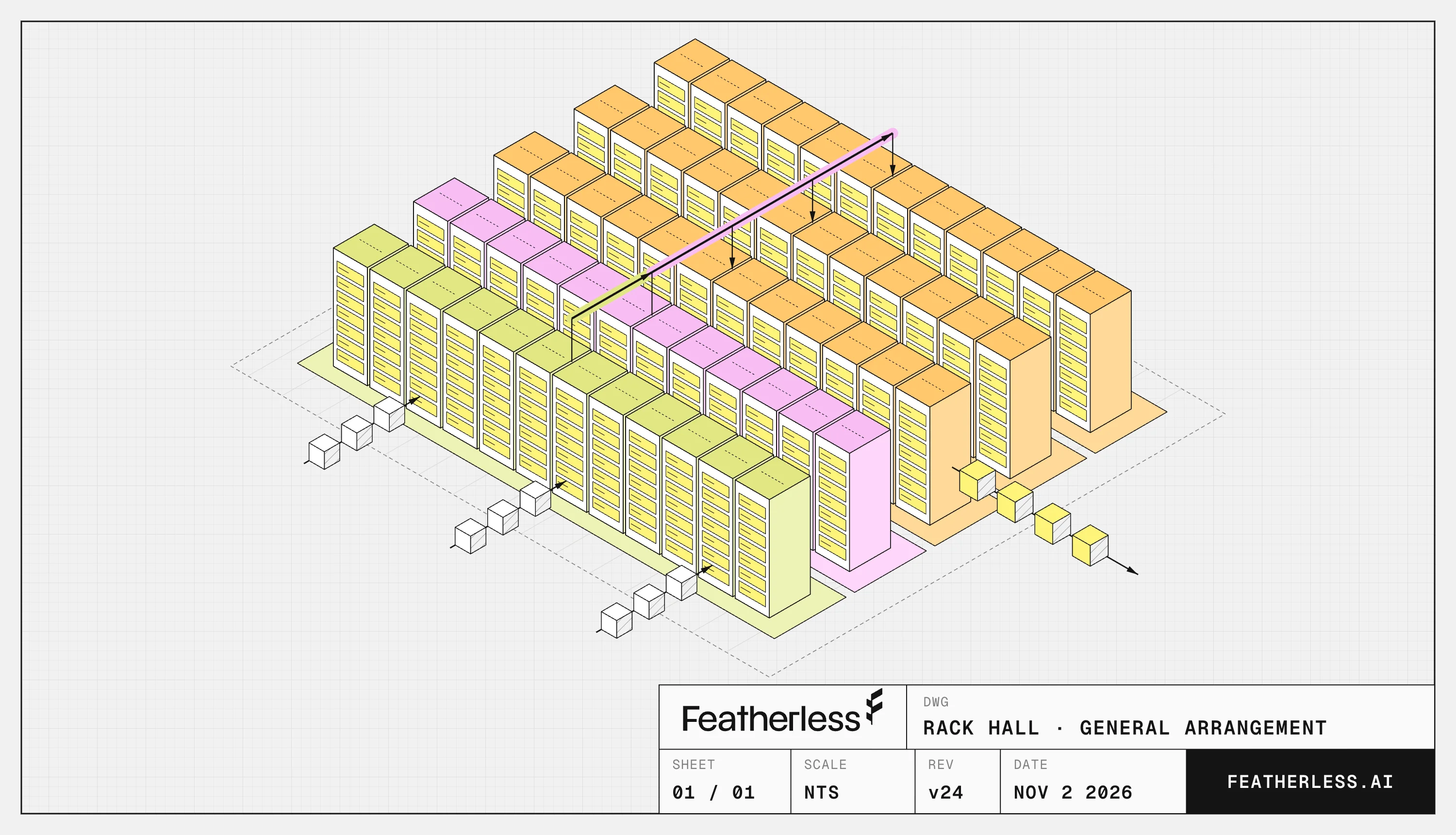
But how do we actually work with this data effectively? The first step is classifying the request, and sending it to the right instance. We use an internal router that checks the size and shape of the prompt, and sends it to a pool configured for that specific workload. Agentic coding traffic typically goes to a pool designed for low latency, while massive prompts get sent to a long context pool. Lastly, requests with lots of images go through their own pool.

Requests of different sizes reach the router, get measured, and go to the pool built for them: speed, long-context or images. Illustrative animation.

Within those pools, we split the work between two different instances. One is the prefill instance (which reads the prompt and builds the KV cache, which is essentially how the model remembers and reuses info from the tokens it’s already processed). The second is the decode instance (which streams the output tokens). They work as a pair. Splitting allows us to tune the two instances to their own job.

Another useful detail that can allow us to optimize further is that the first thousand or so characters of a prompt (the prefix) can be quite similar to each other (for example, popular coding agents will all have similar starting system prompts). We can use this fact to our advantage to enable better routing: the router hashes that prefix and steers requests that start the same way toward the same prefill/decode pair, so the shared part is usually already cached there and can be reused without a trip to our shared cache. We call this hash-bias routing. At sustained load, around 90% of all prompt tokens are read straight from local GPU memory.

If an instance is at capacity, it rejects the request rapidly so the router can walk to the next available one instead of being stuck in a queue.

Sometimes a request can’t go to the pair that already has its cache, for example when that pair is full. This can be a problem, because now the whole conversation would have to get re-read from scratch, which is slow and expensive. To deal with that we use Mooncake, a shared cache that every GPU in the fleet can reach. It’s slower than reading from local memory, which is why hash-bias routing tries to avoid it, but a lot faster than starting from scratch.

Optimize

In the past decade or so, as PCs and phones have gotten more powerful, most software hasn’t needed to squeeze out every drop of performance, and that’s usually fine. This is not the case with AI inference. The demand is through the roof, and there’s a scarcity of compute, which means we have to do everything in our power to optimize our inference stack to an extreme degree.

One way we do this is with quantization, which reduces the precision of the model weights. This can cost accuracy, but with careful testing, we can make sure the model meets its eval criteria while saving enormous amounts of memory, allowing us to serve even more people.

MiniMax M3.1 Flash is a mixture-of-experts model. Each instance runs it in FP4 mode (4-bit quantization) across four MI325X GPUs, on kernels tuned for MI325X, with up to 1 million tokens of context.

We don’t grade ourselves on accuracy. We work with each customer on their own evals and performance targets, and tune the deployment until it meets them. For this customer, that included a tool-calling eval that checks whether the model calls tools exactly right. Our FP4 deployment matches the expected call 98 to 99% of the time across 11 runs, and every query completes.

Stress-test

Now that you’ve chosen a model format and you have a rough understanding of the demands, the next step is to stress-test it. Loading the GPUs is relatively straightforward. The typical numbers we measure are time to first token (TTFT), tokens per second per user (interactivity), and throughput. It’s a balancing act: put more users on the same GPUs and throughput goes up, but each user waits longer and streams slower.

So we stress-tested a 64-GPU slice of the fleet at full sustained load, with prompts ranging from thousands to hundreds of thousands of tokens. Under that load:

• Shorter prompts started streaming in under a second, and even the longest started in under 3 seconds.
• Interactive traffic streamed at around 100 tokens per second per user, with some streams peaking around 185.

Iterate, ship, repeat

We’re still not done optimizing. The last step is an iterative process, driven by AI agents and steered by the inference team, going step by step through each layer of the stack, such as the kernels or vLLM, and making micro-refinements. Each version goes through the same loop: test on a small cluster, roll out gradually, watch the fleet, and so on.

In 12 days, we shipped 32 versions of our inference stack. These can be broken down into 3 phases, with each phase targeting specific parts of the stack that needed refinement.

Phase 1: v1 to v13. v1 was stable but it used twice the amount of GPUs required to meet the customer’s target. Our approach to this was to directly improve the output speed. At v5 we hit the speed target of 60 tok/s per user, with 32 users on two GPUs, and continued to iterate further. By v13, the same traffic was able to run on half the GPUs.

Phase 2: v13 to v20. Decode speed was roughly flat, but this phase focused on improving the p90/p95 TTFT, so that users could have fast, reliable startup times. Under heavy load, the slowest 5% of requests would start about 35% faster in v20 than in v13.

Phase 3: v23 to v32: Here, production moved to four GPUs per instance. Earlier in phase 1 we figured out how to efficiently serve the model. Now, we worked to scale the total throughput that is possible. Each user now gets about 96 tok/s.

What’s next

Just a few years ago frontier models were priced per thousand tokens. Now, we’ve scaled to trillions of tokens, and the demand has continued to increase.

None of this would be possible without our inference team, who built an entire stack around this model in a very short amount of time. We’ll keep sharing what we learn as we go.

If you’re experiencing exploding token demand and need some help, get in touch with us and we’ll create a custom plan for your needs. If you want to build the next generation of inference at scale, we are hiring.

Since you opened this page, counted live at the peak rate.